Chapter 4 Geographic Data

We have introduced the concept of WKT in the previous section, and then we may come up with a few questions: Can R understand WKT format? And how R produce the WKT format from its base code and sf package? In this section, we would first introduce “sf” class and learn the fundamental skill about how geographic data is built. Then, we would further discuss about the transformation of CRS and the method to export the shapefile. Spatial data combines the geometric information and its attributes, and thus, the study on how to join both of them together would be followed by. Please note that, we would use sf package in this section (also the first time to use), and make sure you have this package downloaded (install.packages("sf")).

4.1 Simple Feature Geometries (sfg)

Usually, we have the geographic data in shapefile format downloaded from the website. This allows us to plot the map or do geometric operations without defining the WKT. However, what if we are asked to define the geometric based on WKT format on our own? Simple feature geometries (sfg) helps us to create these objects.

The sfg class contains (multi-)point, (multi-)linestring, (multi-)polygon and geometry collection. A set of functions which start with st_ prefix and end with the name of geometry type create the sfg objects. For instance, st_point() creates the POINT of WKT format. sfg objects can be created from three base R types:

R Data Type	Code	sfg Object
numeric vector	c( )	st_point
matrix	rbind(c( ), c( ))	st_linestring st_multipoint
list	list(rbind(c( ), c( )))	st_polygon st_multilinestring st_multipolygon

Based on the table, we then use the functions of sfg objects to generate geometric information in WKT format.

4.1.1 Point

point_ex=st_point(c(2,3))
class(point_ex)  #identify the data type of sfg object

## [1] "XY"    "POINT" "sfg"

point_ex  #show the WKT format of geometric data

## POINT (2 3)

ggplot(point_ex)+
  geom_sf()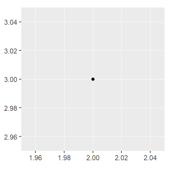

4.1.2 Linestring

linestring_ex=st_linestring(rbind(c(2,3), c(4,4), c(3,5), c(1,4)))
linestring_ex

## LINESTRING (2 3, 4 4, 3 5, 1 4)

ggplot(linestring_ex)+
  geom_sf()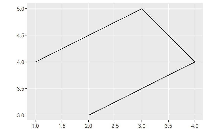

Use rbind to create the matrix, combining all the vector cells (c( )). Note that the connection of line depends on the sequence of the vector cells in the matrix.

4.1.3 Polygon

polygon_ex=st_polygon(list(rbind(c(2,3), c(4,4), c(3,5), c(1,4), c(2,3))))
polygon_ex

## POLYGON ((2 3, 4 4, 3 5, 1 4, 2 3))

ggplot(polygon_ex)+
  geom_sf()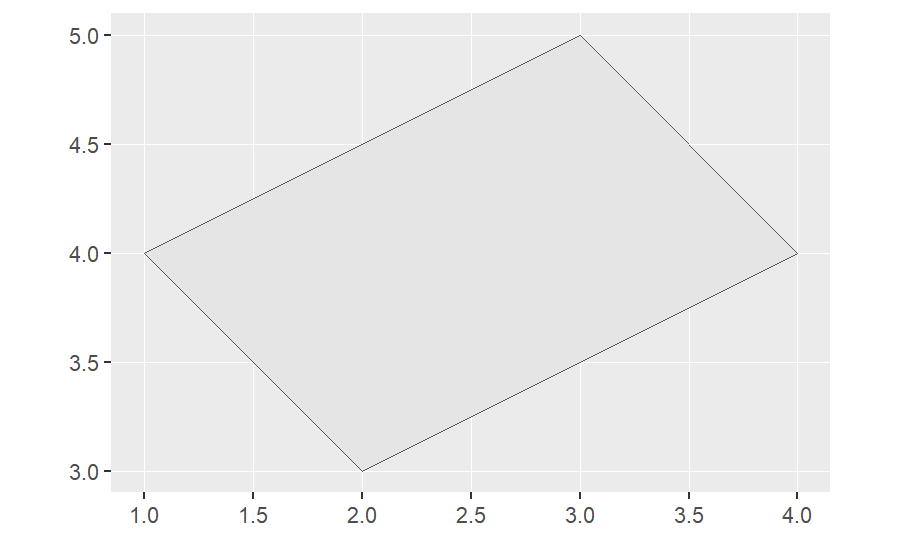

Note that the polygon should be closed, that is, the first vector in the list is the same as the last one.

4.1.4 Multipoint

point_ex=st_multipoint(rbind(c(2,3), c(4,4), c(3,5), c(1,4)))
point_ex

## MULTIPOINT ((2 3), (4 4), (3 5), (1 4))

ggplot(point_ex)+
  geom_sf()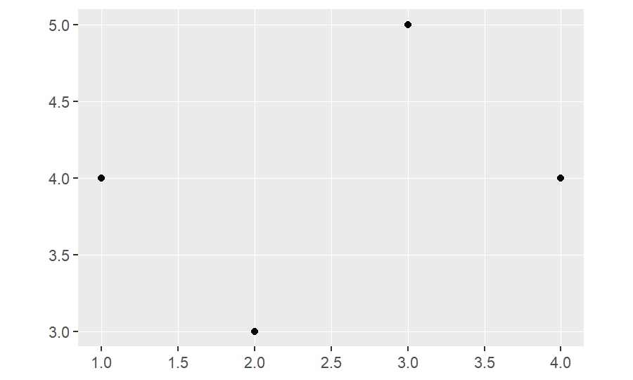

The R data type in st_multipoint is the same as st_linestring, which both of them are matrices.

4.1.5 Multilinestring

linestring_ex=st_multilinestring(list(rbind(c(2,3), c(4,4), c(3,5)), rbind(c(2,5), c(1,2))))
linestring_ex

## MULTILINESTRING ((2 3, 4 4, 3 5), (2 5, 1 2))

ggplot(linestring_ex)+
  geom_sf()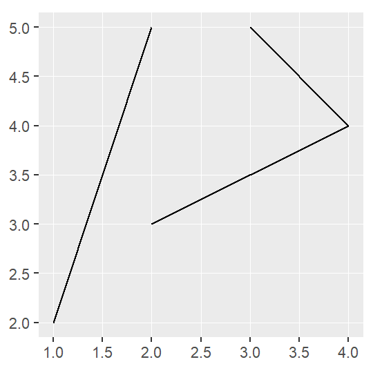

4.1.6 Multipolygon

polygon_ex=st_multipolygon(list(list(rbind(c(2,3), c(4,4), c(3,5), c(1,4), c(2,3))),
                      list(rbind(c(1,5), c(2,5), c(3,6), c(1,5)))))
polygon_ex

## MULTIPOLYGON (((2 3, 4 4, 3 5, 1 4, 2 3)), ((1 5, 2 5, 3 6, 1 5)))

ggplot(polygon_ex)+
  geom_sf()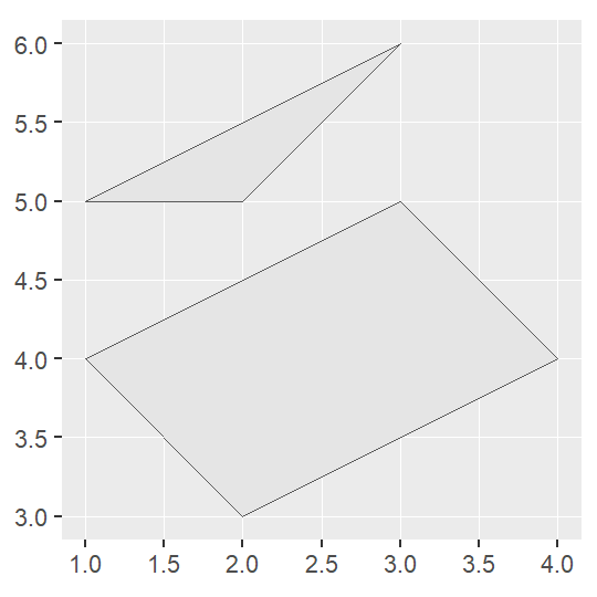

A polygon is created by a list, and thus, multipolygon is generated by a list of lists.

4.2 Simple Feature Columns (sfc)

The sfc object is a list of sfg objects, which additionally contains information about the coordinate system (CRS), geometry type and the border of the whole geometry set (listing the minimum and maximum of x-axis and y-axis). sfc object represents the geometry column in sf data frames.

point_1=st_point(c(2,3))
point_2=st_point(c(4,2))
point_3=st_point(c(1,1))
point_sfc=st_sfc(point_1, point_2, point_3, crs=4326)  #set the CRS to be 4326 (WGS 84)
point_sfc

## Geometry set for 3 features 
## Geometry type: POINT
## Dimension:     XY
## Bounding box:  xmin: 1 ymin: 1 xmax: 4 ymax: 3
## Geodetic CRS:  WGS 84

## POINT (2 3)

## POINT (4 2)

## POINT (1 1)

ggplot(point_sfc)+
  geom_sf()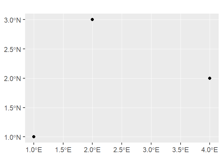

In this example, we can find that the geometry set consists of three points. The border of the geometry set is listed in the bbox (xmin: 1 ymin: 1 xmax: 4 ymax: 3). CRS is set to be EPSG:4326 (i.e.,latitude–longitude system). And please note the axis of the graph. It is labeled as the latitude and longitude format, instead of the integer value labeled in the sfg objects.

If we want to check the CRS and border of the geometry, we can use the functions as follows.

# Check CRS
st_crs(point_sfc)

## Coordinate Reference System:
##   User input: EPSG:4326 
##   wkt:
## GEOGCRS["WGS 84",
##     DATUM["World Geodetic System 1984",
##         ELLIPSOID["WGS 84",6378137,298.257223563,
##             LENGTHUNIT["metre",1]]],
##     PRIMEM["Greenwich",0,
##         ANGLEUNIT["degree",0.0174532925199433]],
##     CS[ellipsoidal,2],
##         AXIS["geodetic latitude (Lat)",north,
##             ORDER[1],
##             ANGLEUNIT["degree",0.0174532925199433]],
##         AXIS["geodetic longitude (Lon)",east,
##             ORDER[2],
##             ANGLEUNIT["degree",0.0174532925199433]],
##     USAGE[
##         SCOPE["Horizontal component of 3D system."],
##         AREA["World."],
##         BBOX[-90,-180,90,180]],
##     ID["EPSG",4326]]

# Check the border
st_bbox(point_sfc)

## xmin ymin xmax ymax 
##    1    1    4    3

4.3 Simple Feature (sf)

The sf object does not only contain the geometry information, but sets of features with attributes. The basic component of its geometry data is sfg, which is recorded in WKT format. Remember the us_states data in package spData? Let’s take a closer look on it. We know that the class of us_states data is not only sf but data frame. A tuple, namely a row, is a simple feature. A simple feature must contain feature attributes and a simple feature geometries (sfg) object, which defines the location of the tuple. The list-column with the simple feature geometries (sfg) for each tuple is then called simple feature columns (sfc).

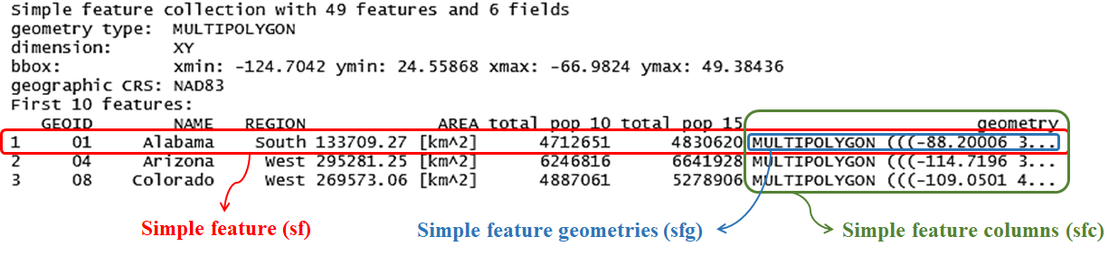
Again, in the figure above, we can find that the geometry type is “multipolygon”. The border of the us_states data is listed in bbox. CRS used in this data is NAD83 (EPSG:4269).

How do we create the simple feature on our own? It is simple, just create the attribute in a data frame, and then use st_sf() function to combine the attributes and the simple feature columns (sfc). There are two parameters should be given in st_sf(). One is data frame, which provides attribute of the features. The other one is geometry, which defines the geometry data that should be based on. If we do not define the CRS in function st_sfc(), then it is required to set CRS in function st_sf().

Example below shows the code to make the simple features of NCTU and NTHU.

uni_geom=st_sfc(
  st_point(c(120.999645, 24.789071)),  # define the sfg of first school (NCTU)
  st_point(c(120.996665, 24.796442))   # define the sfg of second school (NTHU)
  ,crs=4326)  # set the CRS

uni=data.frame(
  name=c("NCTU","NTHU"),               # name of schools
  type=c("university","university"),   # type of schools
  phone=c("03-5714769","03-5712121"),  # phone of schools
  geometry=uni_geom                    # put the sfc into the data frame
)

class(uni)  # the class of "uni" is remain a data frame

## [1] "data.frame"

uni=st_sf(uni, geometry=uni$geometry)  # define the sfc as geometry
# uni=st_sf(uni, geometry=uni$geometry, crs=4326) 

class(uni)  # the class of "uni" changes to data frame as well as sf

## [1] "sf"         "data.frame"

To check whether the class of data we produce is “sf”, we can directly plot the map to confirm it. Let’s recall the tmap function to plot the interactive map.

tmap_mode("view")

## tmap mode set to interactive viewing

tm_shape(uni)+
  tm_dots(size=0.2)

4.4 Convert Text File to Shapefile

In fact, most of the spatial data is stored as shapefile format, which is simple for us to read the files, plot the map and conduct spatial operations in R. However, some spatial data is saved as CSV or XML files. These are not standard geographic data format, and hence, we should convert them in advance. Most of the geometric data they record is under WKT format with pure text (e.g., directly record “POINT (3 2)”). But the function st_sfc() we have learned in the previous section cannot parse the text, whereas it can only identify the vector, matrix, list data type written in R base code. Here, we would introduce a similar function called st_as_sfc, which can help us to read the pure text of WKT.

st_as_sfc("POINT(3 2)")

## Geometry set for 1 feature 
## Geometry type: POINT
## Dimension:     XY
## Bounding box:  xmin: 3 ymin: 2 xmax: 3 ymax: 2
## CRS:           NA

## POINT (3 2)

Also, a function named st_as_text() can retrieve the WKT pure text from the R base data type.

point_ex=st_point(c(3,2))
st_as_text(point_ex)

## [1] "POINT (3 2)"

Knowing the skills of st_as_sfc, let’s take two example data downloaded from government open data, to practice this skill. Data needed has been downloaded previously. You placed the file in the same directory as the R script file. Click here to re-download the file if it is lost.

Let’s use the CSV data named “hsinchu_bus_route” in “csv_files” to produce the bus route map of Hsinchu. There are four columns in this data, including “geometry” columns, which records in WKT format. Use function read.csv() to import the CSV data first.

# read CSV files
BusShape=read.csv("./data/csv_files/hsinchu_bus_route.csv")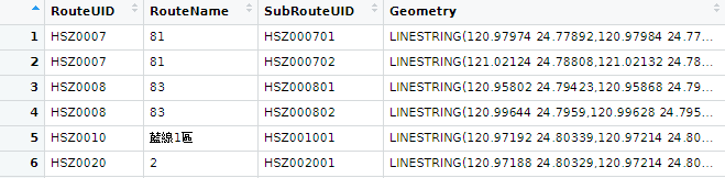

In the CSV data, the spatial feature is listed in the last column named “geometry”. It is recorded as string in the WKT format (LINESTRING()). Then, apply the function st_as_sfc() to convert the column “Geometry” to simple feature columns (sfc). Finally, use function st_sf() to give the data frame with sf class and define its CRS (EPSG:4326).

# convert the column "geometry" to sfc
BusShape$Geometry=st_as_sfc(BusShape$Geometry)

# give the data frame with sf class
BusShape=st_sf(BusShape, crs=4326)

We can use function class() and plot the map to confirm whether we successfully convert CSV file to shapefile.

class(BusShape)

## [1] "sf"         "data.frame"

tm_shape(BusShape)+
  tm_lines()

We are given the geometry directly in WKT format in the example above, so it is easy to transform to spatial data. But what if the data (point) provides longitude and latitude separately in two columns? Here goes an example. We would plot the map regarding scenic spots in Hsinchu. Please import the CSV data named “hsinchu_scenicSpot” in “csv_files” first. There are four columns in the data: ID, Name, PositionLat and PositionLon.

# read CSV files
ScenicSpot=read.csv("./data/csv_files/hsinchu_scenicSpot.csv")
head(ScenicSpot)

##                     ID               Name PositionLat PositionLon
## 1 C1_376580000A_000101 新竹公園(中山公園)    24.80125    120.9771
## 2 C1_376580000A_000029             進士第    24.80947    120.9653
## 3 C1_376580000A_000037         楊氏節孝坊    24.80311    120.9646
## 4 C1_376580000A_000045         香山火車站    24.76312    120.9139
## 5 C1_376580000A_000085       于飛島(鳥島)    24.77494    120.9718
## 6 C1_376580000A_000079   十草原(櫻花草原)    24.76732    120.9379

We need to add a new column (here we name it “geometry”) to paste longitude (X) and latitude (Y) together, and then create the WKT format as POINT(X Y). Use st_as_sfc to convert the column “geometry” to sfc. Last, apply st_sf() to give the data frame with sf class and define its CRS.

# paste the latitude and longitude together, and create WKT text
ScenicSpot=mutate(ScenicSpot, geometry=paste("POINT(", PositionLon, " ", PositionLat, ")"))
head(ScenicSpot)

##                     ID               Name PositionLat PositionLon
## 1 C1_376580000A_000101 新竹公園(中山公園)    24.80125    120.9771
## 2 C1_376580000A_000029             進士第    24.80947    120.9653
## 3 C1_376580000A_000037         楊氏節孝坊    24.80311    120.9646
## 4 C1_376580000A_000045         香山火車站    24.76312    120.9139
## 5 C1_376580000A_000085       于飛島(鳥島)    24.77494    120.9718
## 6 C1_376580000A_000079   十草原(櫻花草原)    24.76732    120.9379
##                          geometry
## 1 POINT( 120.977132   24.801246 )
## 2 POINT( 120.965333   24.809472 )
## 3 POINT( 120.964563   24.803107 )
## 4 POINT( 120.913918   24.763124 )
## 5 POINT( 120.971808   24.774943 )
## 6  POINT( 120.937865   24.76732 )

# convert the column "geometry" to sfc
ScenicSpot$geometry=st_as_sfc(ScenicSpot$geometry)

# give the data frame with sf class
ScenicSpot=st_sf(ScenicSpot, crs=4326)

Use function class() and plot the map to confirm whether we successfully convert CSV file to shapefile.

class(ScenicSpot)

## [1] "sf"         "data.frame"

tm_shape(ScenicSpot)+
  tm_dots(col="red")

4.5 Reproject Geographic Data

After collecting the shapefile data, we may find that their CRS are not consistent, which may cause error in plotting maps as well as in conducting spatial analysis. Hence, it is required to covert them to a same CRS. The inconsistency of CRS often results from the different origin or purpose of the map. In Taiwan, there are two major type of CRS. One is EPSG:4326, which is recorded in latitude and longitude. The other one is EPSG:3826, which is specifically used for the island. However, since shapefiles are managed and released by different sectors (private sector and gonvernment), CRS has not been unified. Function st_transform() can solve this problem by resetting CRS.

We have converted “ScenicSpot” from CSV file to shapefile in EPSG:4326 in the previous section. In the example below, we would further transform CRS to EPSG:3826.

# check the original CRS
st_crs(ScenicSpot)$epsg

## [1] 4326

# transform CRS
ScenicSpot=st_transform(ScenicSpot, crs=3826)

# check the new CRS
st_crs(ScenicSpot)$epsg

## [1] 3826

Let’s compare the data frame of the original one and the new one in the figure below. We can find that the geometry column has been converted based on the CRS.

4.6 Geographic Data Export

We know how to import the shapefile in the previous practice (by function read_sf()). But how to export the shapefile we make in R? By using function st_write, we can export sf data. Two essential parameters should be filled in st_write(): obj means the object we have produced in R; dsn means the directory where we want to save shapefile (the directory should include the name of it and file extension *.shp). Sometimes we have Chinese characters in our shapefile, we should additionally add the parameter layer_options="ENCODING=UTF-8" to ensure that characters would not be garbled.

Let’s again use “ScenicSpot” in the following example. Export the shapefile to the same directory of your R script. You can definitely use absolute path, or simply use relative path to get the same result.

# relative path
write_sf(ScenicSpot, "./ScenicSpot.shp", layer_options="ENCODING=UTF-8")

## Warning in abbreviate_shapefile_names(obj): Field names abbreviated for ESRI
## Shapefile driver

Successfully export the shapefile now? If yes, please check the directory you export to. You may find five files. The file extension includes *.shp, *.shx, *.dbf, *.prj, and *.cpg. The first four files have been introduced in the previous chapter. The last one; however, is in fact not necessary. It is used to specify the code page for identifying the character encoding to be used.

Practically, we may export the data without the geometry information, and only retain the attribute of the shapefile. In this situation, we need to first use function st_drop_geometry() to retrieve the attribute data of a simple feature, and simply use function function write.csv() to export it. Take data us_states for example. It is originally a simple feature with geometric information. The code to export the attribute information is shown below.

# get rid of the geometry first
us_states_attr=st_drop_geometry(us_states)

head(us_states_attr)

##   GEOID        NAME   REGION             AREA total_pop_10 total_pop_15
## 1    01     Alabama    South 133709.27 [km^2]      4712651      4830620
## 2    04     Arizona     West 295281.25 [km^2]      6246816      6641928
## 3    08    Colorado     West 269573.06 [km^2]      4887061      5278906
## 4    09 Connecticut Norteast  12976.59 [km^2]      3545837      3593222
## 5    12     Florida    South 151052.01 [km^2]     18511620     19645772
## 6    13     Georgia    South 152725.21 [km^2]      9468815     10006693

# export the attribute
write.csv(us_states_attr, "./us_states_attr.csv")

4.7 Geographic Data Format

Up to now, we learn how to import and export the shapefile. But is it true that R can only cope with the shapefile format? Apparently not! There are in fact several formats we have not discussed in the past section. Here, we would like to introduce some important geographic data formats that are commonly used in spatial analysis.

Shapefile is the most popular vector data format. However, it has some limitations listed below:

1. It is a multi-file format, which consists of at least three files.
   
2. It only supports 255 columns and the file size is limited to 2 GB.
   
3. It is unable to distinguish between a polygon and a multipolygon.

In spite of the limitations, we are still inclined to use shapefile, and lots of data provided by government use it. Aside from shapefile, Geopackage is a format for exchanging geospatial information. It defines the rules on how to store geospatial information in a tiny SQLite container. Hence, GeoPackage is a lightweight spatial database container, which allows the storage of vector and raster data. KML (Keyhole Markup Language) is an XML notation for expressing geographic annotation and visualization within two-dimensional maps and three-dimensional Earth browsers. It was developed for use with Google Earth. GeoJSON is an open standard format designed for representing simple geographical features, along with their non-spatial attributes. It is based on the JSON format. GPX (GPS Exchange Format) is an XML schema designed as a common GPS data format for software applications. It can be used to describe points, tracks, and routes.

If we want to export the geographic data in those formats, just simply change the file extension in the directory. Take “ScenicSpot” we produce again, and generate the spatial data in GeoPackage format.

# relative path
write_sf(ScenicSpot, "./ScenicSpot.gpkg")

# import the data and check if it is successfully generated
read_sf("./ScenicSpot.gpkg")

## Simple feature collection with 94 features and 4 fields
## Geometry type: POINT
## Dimension:     XY
## Bounding box:  xmin: 239280.7 ymin: 2737355 xmax: 251527.1 ymax: 2749333
## Projected CRS: TWD97 / TM2 zone 121
## # A tibble: 94 x 5
##    ID                   Name           Posit~1 Posit~2               geom
##    <chr>                <chr>            <dbl>   <dbl>        <POINT [m]>
##  1 C1_376580000A_000101 新竹公園(中山~    24.8    121.   (247688 2743764)
##  2 C1_376580000A_000029 進士第            24.8    121. (246495.3 2744675)
##  3 C1_376580000A_000037 楊氏節孝坊        24.8    121. (246417.3 2743970)
##  4 C1_376580000A_000045 香山火車站        24.8    121. (241294.3 2739544)
##  5 C1_376580000A_000085 于飛島(鳥島)      24.8    121. (247149.1 2740851)
##  6 C1_376580000A_000079 十草原(櫻花草~    24.8    121. (243716.3 2740007)
##  7 C1_376580000A_000007 新竹都城隍廟      24.8    121. (246528.1 2744113)
##  8 C1_376580000A_000042 鄭用錫墓          24.8    121. (247062.5 2742288)
##  9 C1_376580000A_000027 消防博物館        24.8    121. (246781.4 2744342)
## 10 C1_376580000A_000044 新竹神社殘跡(~    24.8    121. (245226.6 2742840)
## # ... with 84 more rows, and abbreviated variable names 1: PositionLat,
## #   2: PositionLon

4.8 Join Attribute and Spatial Data

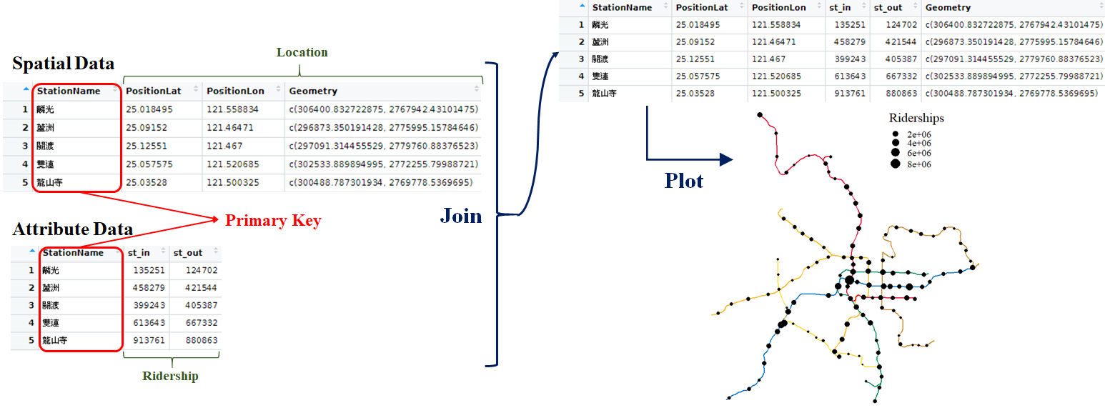
In reality, most of the attribute features we want to analyze and spatial feature are not in the same file. Usually, the spatial features are stored as shapefile format, while the attribute features are provided in a CSV or spreadsheet file. Take transportation data for instance. If we want to plot the map showing the number of passengers getting on and off at each MRT stations, we need spatial features recording the location of each stations, and attribute features recording the ridership counts. In this example, the geometry data (shapefile) can be downloaded from GIS-T website, while the operating data (spreadsheet) can be derived from Taipei Rapid Transit Corporation. Apparently, the data management agency and the format of two data are not consistent. Hence, combining data from different sources would be a vital and common task before the spatial analysis.

A primary key is required among the data to be joined. Primary key is a specific choice of a minimal set of attributes (columns) that uniquely specify a tuple (row) in a table. In other words, primary key is a common column that can help us link the spatial features to attribute features. In the MRT example we have mentioned above, the primary key between spatial and attribute data may be “MRT station name” or “MRT station ID”. The procedure of join is illustrated in the figure below.

Now, let’s join the data provided in package spData. “world” is simple feature data that stores the geometry of the shape of each country. “coffee_data” is a data frame which records the production of coffee in every nations each year. We want to join two data together, and perform the map about the world coffee production by country. Use function left_join() to accomplish our goal. In left_join(), the first data placed would be on the left-hand side of the new data frame; while the latter one would be on the right-hand side. Parameter by="" should be given if the column is specifically to be joined, or the function would join the data based on all the columns that have common name by default. In this example, the primary key is the country name. The column name in both data are the same, which is named “name_long”. The code and result are shown below.

# join the spatial and attribute features
world_coffee=left_join(world, coffee_data, by="name_long")

# print the result
world_coffee[,c("name_long","continent","coffee_production_2016","coffee_production_2017")]

## Simple feature collection with 177 features and 4 fields
## Geometry type: MULTIPOLYGON
## Dimension:     XY
## Bounding box:  xmin: -180 ymin: -89.9 xmax: 180 ymax: 83.64513
## Geodetic CRS:  WGS 84
## # A tibble: 177 x 5
##    name_long        continent     coffee_pro~1 coffe~2                      geom
##    <chr>            <chr>                <int>   <int> <MULTIPOLYGON [arc_degre>
##  1 Fiji             Oceania                 NA      NA (((-180 -16.55522, -179.~
##  2 Tanzania         Africa                  81      66 (((33.90371 -0.95, 31.86~
##  3 Western Sahara   Africa                  NA      NA (((-8.66559 27.65643, -8~
##  4 Canada           North America           NA      NA (((-132.71 54.04001, -13~
##  5 United States    North America           NA      NA (((-171.7317 63.78252, -~
##  6 Kazakhstan       Asia                    NA      NA (((87.35997 49.21498, 86~
##  7 Uzbekistan       Asia                    NA      NA (((55.96819 41.30864, 57~
##  8 Papua New Guinea Oceania                114      74 (((141.0002 -2.600151, 1~
##  9 Indonesia        Asia                   742     360 (((104.37 -1.084843, 104~
## 10 Argentina        South America           NA      NA (((-68.63401 -52.63637, ~
## # ... with 167 more rows, and abbreviated variable names
## #   1: coffee_production_2016, 2: coffee_production_2017

# plot the map (use 2017 data)
ggplot(world)+
  geom_sf(fill=NA)+
  geom_sf(data=filter(world_coffee, !is.na(coffee_production_2017)), aes(fill=coffee_production_2017))+
  scale_fill_continuous(low="#F2E6E6", high="#984B4B")+
  theme(panel.background=element_blank())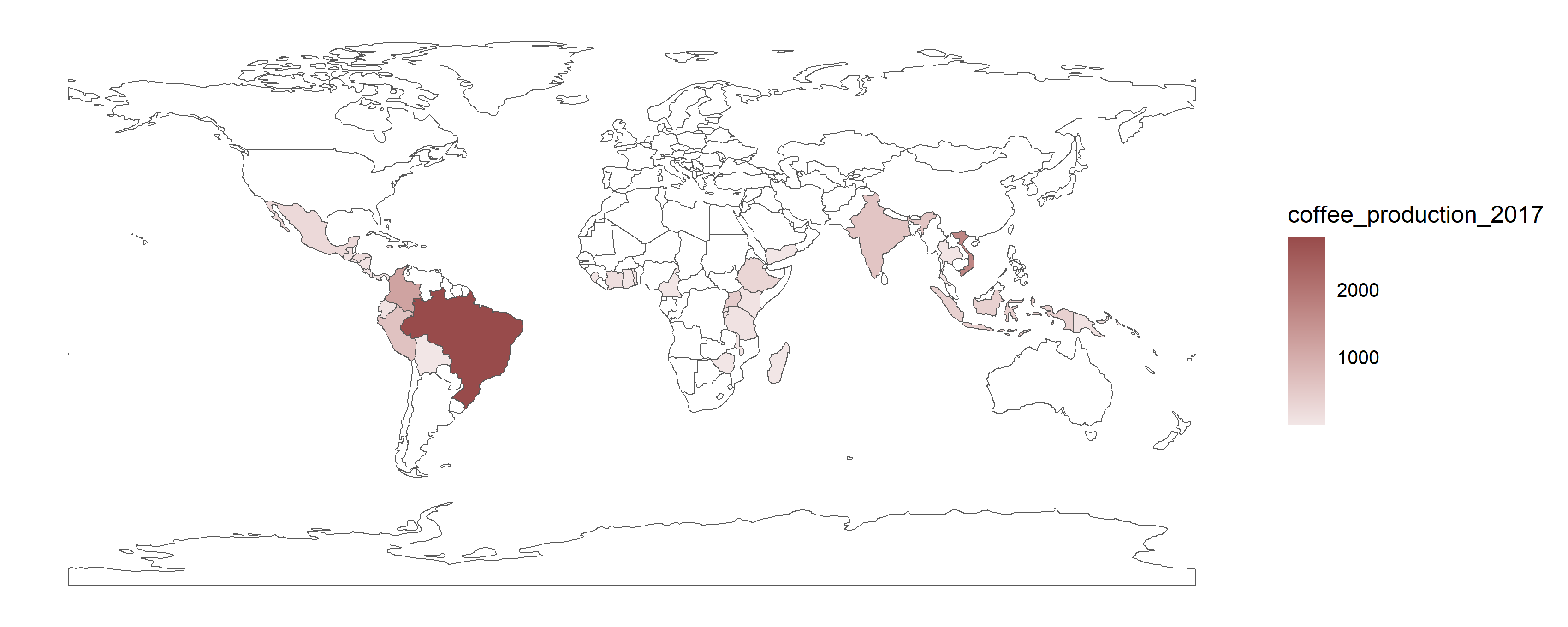

In the section above, we repeatedly show the method of how to connect the spatial features and attribute features. But actually, for some practical reasons, we tend to drop the geometry object from the data. Use the function st_drop_geometry() can do so. Take “ScenicSpot” data again. It is now with spatial features, and we can apply this function to eliminate the geometry.

# check the class of ScenicSpot
class(ScenicSpot)

## [1] "sf"         "data.frame"

ScenicSpot=st_drop_geometry(ScenicSpot)
head(ScenicSpot)

##                     ID               Name PositionLat PositionLon
## 1 C1_376580000A_000101 新竹公園(中山公園)    24.80125    120.9771
## 2 C1_376580000A_000029             進士第    24.80947    120.9653
## 3 C1_376580000A_000037         楊氏節孝坊    24.80311    120.9646
## 4 C1_376580000A_000045         香山火車站    24.76312    120.9139
## 5 C1_376580000A_000085       于飛島(鳥島)    24.77494    120.9718
## 6 C1_376580000A_000079   十草原(櫻花草原)    24.76732    120.9379

# check the class of ScenicSpot again
class(ScenicSpot)

## [1] "data.frame"

4.9 PRACTICE

In this chapter, we have learned the concept of the spatial features as well as attribute features, and show some examples about the method to join the data. Now, it’s time for you to practice the three skills on your own.

• Set up simple features.
  
• Join the spatial and attribute data.
  
• Plot the map. (Review previous chapter)

Data needed has been downloaded previously. You placed the file in the same directory as the R script file. Click here to re-download the file if it is lost.

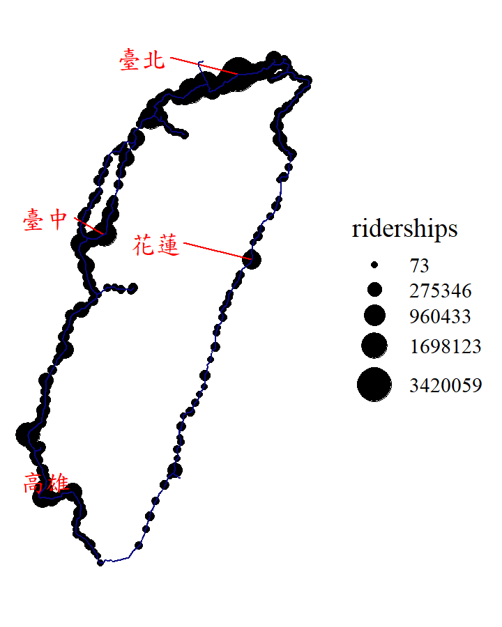
Three data needed in the example is stored in the file “TRA”. “TRA_line” records the name of railway line and its geometry (WKT format), whereas “TRA_station” records the name of train station and its longitude and latitude. Ridership data of November, 2020, is stored in “TRA_ridership”. We want to plot the map of the route and station of Taiwan Railway Administration (TRA). The data provided is not in shapefile format, but the CSV files. You should convert it to the simple features in advance based on the skills you have learned. Additionally, please join the data of train station and ridership of each station. Last, plot the map, and the size of point of station should be based on the number of ridership, that is, the station with more ridership should be larger point.

First of all, since the ridership data is given by date for each stations, we need to sum up all the ridership based on the station before joining the data. We would like to use package dplyr to tidy it.

# read the ridership data
ridership=read.csv("./data/TRA/TRA_ridership.csv")

# the ridership is given by date for each stations
head(ridership)

##   trnOpDate staCode gateInComingCnt gateOutGoingCnt
## 1  20201101     900            8063            7635
## 2  20201101     910            1054            1053
## 3  20201101     920            1732            1775
## 4  20201101     930            4225            4300
## 5  20201101     940            1938            1901
## 6  20201101     950            1434            1331

# group by and summarize the data
ridership=group_by(ridership, staCode)%>%
  summarise(riderships=sum(gateInComingCnt+gateOutGoingCnt))

# print the final result
ridership

## # A tibble: 239 x 2
##    staCode riderships
##      <int>      <int>
##  1     900     438926
##  2     910      80125
##  3     920     131957
##  4     930     360184
##  5     940     157416
##  6     950     115831
##  7     960     620925
##  8     970     582197
##  9     980     704605
## 10     990     960433
## # ... with 229 more rows

The rest of the work would be done on your own. Here comes with some tips:

1. Please note that the data “TRA_line” and “TRA_station” contain Chinese character, so make sure to add fileEncoding="UTF-8" in read.csv().
2. Please use EPSG:4326 as CRS, which is in longitude-latitude form.
   
3. Please note that the TRA station code in two data are not the same type. One is numeric, and the other is character. It is recommended to transform all the station code to numeric type. (If the type of station code is not unified, the error would be shown in left_join().)
4. As the column name of data should be joined is not the same, you should define the parameter by="" in the following forms: by=c("A"="B"). “A” means the data you place in the first parameter in left_join(), while “B” means the data placed in the second parameter.

The result is shown below.